In this video I'll demonstrate the basic features of Google Colaboratory. It's not my goal here to show you absolutely everything it can do, because we're still just getting started, but you should know the basics so that you can start benefitting from this tool as soon as possible.

Open a new notebook

To get started, let's open up a new notebook together.

In your web browser, go ahead and navigate to colab.research.google.com and then click on the New Notebook button.

This will automatically create a new Google Colab document within your Google Drive. This document you see here is called a "notebook". Google automatically gives the notebook a title of something like "untitled##.ipynb". The file extension .ipynb stands for IPython Notebook. Now, That's not something you need to remember, but hopefully that makes the file extension mean something to you when you see it again in the future.

Let's give our document an actual title, you can call yours whatever you like, I'm going to call mine intro_notebook.ipynb.

What is a notebook?

Next we're going to focus on this middle section of the document. This is where all of the action happens. A notebook is made up of a bunch of what are called "cells", and there are two types of cells. There are "text cells" and "code cells". Now when you hear the word "cell" I just want you to think "section", right? This document is going to have some code sections and some text sections.

Code Cells

In the code cells we'll write Python code to analyze and clean our data, fit machine learning models, all that fun stuff. Learning what to write in the code cells and the process for properly preparing and modeling our data is the bulk of what we're going to be learning in future lessons and courses.

Whenever you open a new notebook it will always start off with one code cell already created within it. Go ahead and click on it and type print("hi").

Let's run the code cell by clicking on the play button on the left-hand side. Now that we've run some Python code, we can see that a code cell itself is made up of two sections –an "input section" and an "output section".

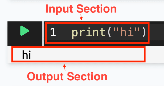
The input section is where we write our code. The output section is the area beneath the code where we see the word hi. Our code won't always generate an output, but often we'll intentionally cause things to be shown here to make sure that our code has run successfully and that our program is doing what it should be.

Adding New Cells

Let's add a new text cell to our document. You can add new cells either by hovering over the section immediately before/after a cell...

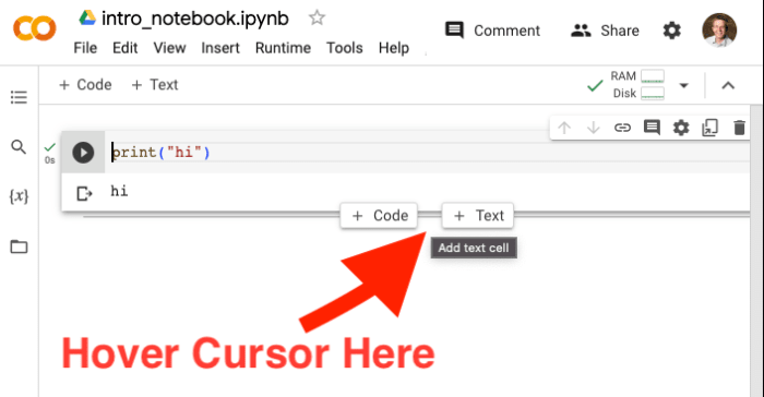
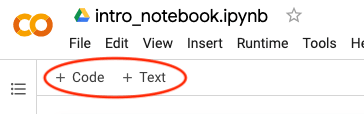
or by using the + Code or + Text buttons on the left-hand side just below the main menu.

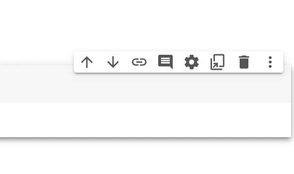
If you accidentally add more cells than you want or have them in the wrong order, you can delete any unwanted cells or rearrange the order of the cells using the buttons on the top-right of any cell.

Text Cells

Let's make sure that our text cell comes before the code cell, and then we'll add some content to it. In text cells, we document our work. We'll often be sharing our notebooks with others, so it's important that we explain what we're doing so that others can follow along.

Text cells operate using a markup language called "Markdown". Markdown is a system for controlling the structure and formatting of documents –and it's really nice because all it takes is addition of a few symbols to make our document look professional. We write markdown as plain text but then the symbols that we add to it get interpreted by the computer and rendered into the version that readers end up interacting with.

To show you what I mean, let's edit a text cell. Double click on it to begin editing. You can also select it with a single click and then hit enter. I find myself double-clicking most often.

Let's go over some of the basics of Markdown. I'll link to a full Markdown Cheat Sheet below the video.

As you type in a code cell, Colab will automatically generate a preview of the rendered version of your markdown here on the right.

You'll see that on the left side I'm just typing plain old text, but if I add a pound sign # at the beginning of the line (some of you may know this symbol as a "hash tag"), then our text will be transformed into a large "heading". The more pound signs we add the smaller the heading will be.

If I want just a regular paragraph of text then I don't add any pound signs at the front of it.

We can also easily italicize and bold words. A single set of asterisks or underscores will cause the words to be italics and a double set of asterisks or underscores will cause the text to have a bolded font.

We can create a bulleted list by beginning each newline with a dash.

Or we can create an ordered list by starting each newline with a number and a period

We can easily turn any text into a link by wrapping the text that we want to serve as the active link in square brackets, and then immediately following the closing square bracket we'll put a pair of parentheses. Inside of the parentheses we put the URL that we want to link to.

We can even insert an image using in almost the same way. The biggest difference is that we put an exclamation point just before the opening square bracket. And in this instance the text that we put in the square brackets will become the "alt text" of the image. Alt text is important so that individuals who have impaired vision and also search engines can get an idea of what is in an image without actually viewing it. So we want the alt text to describe what's in the image.

In order for an image to show we need a link to the image. This can usually be found by first finding the image that you want to embed shown in a webpage. And then you can right click on it and say "Copy Image Address" or, you can click on the "Open Image in New Tab" option and then just copy the URL from the browser's URL bar. If we drop the link to the image inside of the parentheses the image will appear. The first time I did this I was shocked by how easy it was to embed an image in markdown.

If we want to format something as code we will wrap it in "tick marks". The tick mark symbol is found on your keyboard just to the left of the number 1. It shares a key with the tilde symbol ~.

If we want to showcase a large block of code then we can do the same thing but using a set of triple tick marks instead. We can also add code syntax highlighting by writing the name of the programming language represented in the code immediately after the opening trio of tick marks.

There's also blockquotes, horizontal rules, footnotes, and tables. Tables require a bit of typing, I've got one prepared here that I'll copy-paste into the document instead of making you watch me type it all out. If you want to add tables like this, I recommend using a Markdown table generator tool so that you don't have to type all of this manually. I'll link to one that I like below the video.

And that's the basics of using Markdown within text cells. Text cells have a few other tricks up their sleeves, but what I've shown here is more than enough to get your started.

Demonstration

Now that we've covered a lot of the most important aspects of text cells I've got a few more features of notebooks that I want to show you. Let's explore them by doing something fun in this notebook.

Now, just a heads up. I'm going to write some of code in this next demonstration, and I just want to emphasize that I DO NOT expect you to fully understand or follow along with the code I'm about to write. What I want you to focus on is what our notebook document is doing.

What Python Packages Does Google Colab Have Installed?

In the previous video you'll remember that I talked about how Google Colab is a cloud-based notebook editor because it talks to and runs all of our code not on our own computers but instead on a computer at a Google datacenter. You'll also recall that part of what's so great about Google Colab is that it comes with all kinds of pre-installed Python Packages that are ready for us to use –out of the box– so that we don't have to worry about any setup.

Well, I want to use one of these pre-installed Python Packages to give you a very small taste of what it's like to work with actual data in a notebook –but more importantly, I want to demonstrate some of the most important features of Google Colab.

I'm going to remove all this stuff from the text cell and just add a header that says # Making a Graph with Seaborn because that's what we're going to end up doing together.

Let's also delete the print statement from our code cell and replace it with the following:

!pip freeze

When we run the cell, this line of code will cause all of the tools that Google Colab has (and their version numbers) to be displayed in the output section of the code cell. Just take a look at this list, there's all kinds of stuff here. In particular, there are some familiar names like numpy, pandas, matplotlib, scikit-learn, tensorflow, and many others. The gang's all here –as they say.

Clearing Long Code Cell Output

By the way, you see how the output section of this code cell is really long? If I find that the output section of the code cell is so big that it's in my way while I'm working I can click on the three dot icon on the far-right of the code cell and then select "Clear output" from the dropdown menu and that will remove the output section of the code cell. If I want to get it back I'll need to run the code cell again.

Keyboard Shortcuts

Before we start using one of these juicy tools, I want to take this opportunity to point out that there are a lot of useful keyboard shortcuts that you can use to speed up your work in Google Colab. But for starters, there's one in particular that I want you draw your attention to.

If I have a code cell selected, and I hold shift and then hit enter that will automatically run the code cell and move me down to the next cell below it. That way you don't have to leave your keyboard and go to your mouse to click the play button every time. Just a helpful tip.

If you use this keyboard shortcut while you have a text cell selected, it will close down the text cell editor and move you down to the next cell.

Making a Graph with Seaborn

1) Importing the Seaborn Graphing Library

You'll see in the list of available packages here a tool called "Seaborn". We're going to use it to load a dataset that comes along with Seaborn and make a colorful graph as a small demonstration here.

The first step when working with a Python Package is to import it into our notebook. Write import seaborn as sns and then run the code cell. Now Seaborn is ready for us to use. the as sns part of this line of code means that we can refer to this tool as sns in our code as an abbreviated form of its name.

import seaborn as sns

2) Load the Dataset

The dataset that I want to work with is called the "Palmer Penguins" dataset. It's one of my favorite so-called "toy datasets" . The Palmer Penguins dataset holds information about three different species of penguins. For each penguin listed in the dataset we have the Penguin's species, the Island they were found on, some measurements of their bill and flippers, their weight, and the sex of the animal.

Here, we'll even include an image of the three penguin species in our first code cell to liven up the notebook.

Let's go ahead and load the dataset by running:

df = sns.load_dataset("penguins")

df here stands for "dataframe". A dataframe is basically fancy table that holds our data and helps us work with it.

In the the next code cell go ahead and write df.head(). df.head() will display for us the first 5 rows of the dataset. This is one example of us causing something to be displayed in the output section of the code cell so that we can verify to ourselves that the dataset truly has been loaded and that everything looks to be in order.

df.head()

Very cool. I hope this helps you get an idea of what the data looks like.

Don't be Afraid to Look Stuff Up!

Next, I want to make a fancy graph with this data called a "pairplot". But, we're going to pretend that I've forgotten how to do it. I want to show you a couple of the ways that Google Colab can help jog our memory if we know that a tool exists, but can't remember exactly how to write the code for it.

And I want to emphasize that this is a common situation that you'll find yourself in. A lot of beginner data scientists are quickly overwhelmed by all of the different tools that we use. New learners often make the mistake of trying memorize everything and remember how exactly to use each tool that they've ever brushed up against, but there's just too much to be able to memorize it all. The things that are worth remembering you will naturally memorize over time because you'll do them so often.

Even the most senior data scientists have look to things up –constantly. It's a regular part of the job. So don't feel like a failure if you have to look something up.

How to Look Up Documentation in Google Colab

There are three different methods of looking up documentation that I want to make you aware of.

Say that from memory I know that I want to make a pairplot graph using the seaborn library and that's all that I can really remember. A helpful tool that I can use is something called the help() function type out help() and then inside of the parentheses put the name of the whatever you want help with.

help(sns.pairplot)

This will pull up the official documentation for pairplot and display it in the output section of the code cell. This documentation probably won't make a whole lot of sense to you right now, don't worry about that. We'll get really good at reading documentation as time goes on.

A second method that I like a little bit better than this is to type sns.pairplot but then to just put a question mark at the end of it. This will pull up the same documentation but will put it in this convenient sidebar. It's really up to you which of these two methods you prefer. Try both and see which method you like best.

sns.pairplot?

However, my favorite method of looking up documentation doesn't have to do with notebooks at all. I like to just google for the thing that I'm trying to do. There will always webpages that also host the tool's official documentation –made by the creators of the tool. There's posts on a forum called StackOverflow that might be helpful, or just blog posts and other tutorials out there that have been made by kind individuals. Getting good at googling things when you get stuck or can't remember something is a really important skill to develop.

So let's google "seaborn pairplot" and I'll show you why this is my preferred method for looking up documentation. Here we see the official Seaborn documentation for Pairplot. You'll notice that the text on the page here is pretty much exactly the same text we saw using the help() function and question mark methods. But, in my opinion, the text here has been formatted a little bit nicer and is easier to read. But that's not the best part. If we scroll to the bottom here there are usually code examples of how to make this graph. These are really valuable to me and they're typically not included when we use the help() or ? method.

Making a Graph with Seaborn

From this documentation I would learn that I should type "sns.pairplot" then parentheses, and then I put the name of the dataframe inside of the parentheses. In our case we've called our dataframe df.

And there we go, we've made a graph! You'll notice that the graph shows up in the output section of the code cell. And it looks good!

sns.pairplt(df)

Now, if we revisit the documentation, you might get an idea for what it's trying to tell us here. All of these parameters here, like "hue", "hue-order", "palette", "vars", "kind", etc. are other settings that we can use to control how our graph looks. Don't worry if that didn't jump out at you from the documentation here, again, reading and understanding documentation is a skill that we're going to practice a lot, and this documentation won't make very much sense until we learn more about how to write code with Python.

Let's add hue='species' to our pairplot and see how that changes what it looks like. Now, If you look closely at the Seaborn documentation, you'll notice that they're also using the Palmer Penguins dataset in their code snippets at the bottom of the documentation. Which is part of why I chose to use that dataset for our demonstration.

sns.pairplot(df, hue='species')

I also want you to notice that this graph is displayed in the output section of our code cell. The ability to create graphs like this and for them to be displayed within the notebook immediately after the code that created them is another advantage of notebooks over other code writing tools. Graphs and visualizations can be effective communication tools –if used wisely– and they also add some visual flare to our work.

A Notebook's "Hidden State"

Next I want to go over one of the biggest points of confusion for new learners when it comes to notebooks. Here in the top menu you'll see a Runtime button. And below that there is a 'Restart Runtime" option. Go ahead and click on it. This little warning pops up here. We're going to say that "yes" we're sure that we want to restart the runtime.

When we do that you'll notice that in the top right that the notebook shows itself rebooting more or less. And that the little numbers that used to be next to every code cell have disappeared, but that none of our code cells or text cells have been affected. Even the graph is still there.

If none of our cells were affected, what was the point of Google Colab warning us that things were going to get deleted? If we make the popup appear again, we'll see that it said that "Runtime state including all local variables will be lost." Well what is this so-called "runtime state" also sometimes referred to as "hidden state"?

How to view our notebook's hidden state

As we write code we'll often do things both intentionally and unintentionally that will cause things to be stored within our notebook's internal memory. That's essentially what this "hidden state" is.

Let's think about it.

Re-run the code cells up to that point where we loaded the dataset and then click on this {x} –x surrounded by curly braces– button in the left-hand sidebar. This "variable inspector" panel –as it's called– tries to help us see our notebook's internal storage.

When I loaded the dataset this equals sign told the dataset to store itself within my notebook under the name df. This stored the penguins dataset in a way that it could be retrieved from the notebook's memory whenever we use the variable df –and we can see the df variable listed in the left-hand sidebar. This is why we continued to use the variable df in the next code cell where we ran df.head(). We essentially said, hey pull up that dataset from the notebook's memory and show me its first five rows.

Let's restart the runtime yet again, but this time skip down and try to immediately run the df.head() code cell and see what happens. This time, we get an error message saying that name 'df' is not defined. When we restarted the runtime, we didn't change any of the cells in our notebook, but we did wipe out our notebook's hidden state. We can't look at the first 5 rows of the notebook because the dataset has been removed from our notebook's internal memory.

The little numbers on the side of each code cell were trying to tell me that I had skipped some potentially important code cells, and that's one way that I could have recognize my mistake. These numbers on the left-hand side of each code cell are very important. They're called the execution count and they indicate to us the order in which the code cells were run. Which brings me to the really important point that I wanted to get to:

In a perfect world, notebooks would be run from top to bottom executing each cell exactly one time.

However, when we're drafting the document and working on it that's usually not how we interact with the notebook. We're usually jumping around editing things and trying things out. And sometimes when we run code cells out of order, funky things can happen to our notebook's internal storage. Things can get mixed up. I want you to be aware of this potential pitfall because sooner or later as you're working with a notebook weird things are going to start happening as a side effect of the order that the code cells have been run in. When that happens here's what I want you to do.

First, double check the numbers on the left-hand side of each code cell to make sure that you haven't accidentally forgotten to run a cell or have run the cells out of order. Sometimes even running the same cell multiple times can cause problems.

Second, if the problem persists, restarting the runtime and then re-running the code cells from top to bottom will usually iron out any weird behavior. This is the notebook equivalent of common IT advice to "turn it off and on again".

When you're done with your work and ready to share your notebook with others, it's a best practice to restart the runtime and then run each of the cells in order just to make sure that everything's working properly –or you can just use the "Restart and run all" option from the dropdown menu.

Accessing Local Files in Google Colab.

Because Google Colab is a cloud-based notebook editor that means that a google datacenter computer is serving as the filesystem for our notebook. So, if we want our notebook to have access to files on our local machines, we'll need to do a little bit of extra work and upload any necessary files from our local computer to this specific Colab Notebook.

On the left-hand sidebar you'll see a folder icon. Go ahead and click on it. This has opened up what's called "files pane" where we can upload files that we want our notebook to have access to.

Click on the "upload" button to select a file from your local computer. Files that you upload will only be available while the notebook's runtime is active, so if you close this tab in your browser or step away from your machine for a long period of time and your runtime shuts down, you might need to re-upload the file(s).

After you've uploaded a file you might need to click on the refresh button (that's just to the right of the upload button) in order for the filename to show up in the sidebar.

We could have almost-as-easily used the files pane to upload a CSV file of the Palmer Penguins dataset and then loaded the CSV to a dataframe in a code cell, but I don't want to distract you –any more than I have to– with code that's foreign to you during this lesson. I mostly just want to make you aware that the files pane can be used to upload local files.

Sharing Notebooks With Others

One of the big benefits of working in Google Colab is that because this document lives in our Google Drive, we can share it with others just like we would any other Google Drive Document. In the top right corner click on the "Share" button and you'll see that we have the option to share this notebook with specific individuals by adding their email address or we can also create a shareable link to the notebook.

If you're ever stuck on something and you need to ask for help, it's a good idea to put the code that you're working on in a notebook in a way that reproduces the problem you're experiencing and then to share a link to whomever you're asking for help. That way they can easily see your code, review what you've done and give you any necessary pointers.

Wrapping Up

The most important skillset that I hope you start emphasizing in yourself as a result of this video is getting good at looking things up and using references to refresh your memory when you forget something –and don't beat yourself up about it.

This is part of why you having familiarity with Google Colab –right from the get-go– is so important. I hope that you will use this tool not only to do your core data science work, but also to create references and cheat sheets for yourself. If there's something that you find yourself looking up often, make a notebook about it explaining to yourself how that tool works. Not only will this help you learn more thoroughly whatever it is that you keep on forgetting, but having those additional references will help you be productive and efficient in your work.